20天狂宴Pytorch-Day8

GitHub链接

低阶 API, 中阶 API, 高阶 API, 登神长阶 API.

低阶 API

线性回归模型

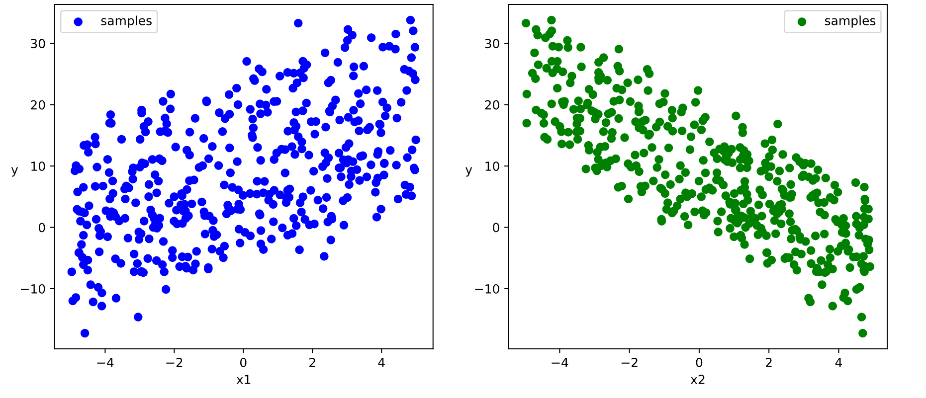
生成随机测试数据.

n = 400
X = 10*torch.rand([n,2])-5.0	# torch.rand是均匀分布 
w0 = torch.tensor([[2.0],[-3.0]])
b0 = torch.tensor([[10.0]])
Y = X@w0 + b0 + torch.normal(0.0,2.0,size = [n,1])	# @表示矩阵乘法,增加正态扰动

数据大概长这样.

接下来构建数据管道迭代器.

def data_iter(features, labels, batch_size=8):
    num_examples = len(features)
    indices = list(range(num_examples))
    np.random.shuffle(indices)	# 样本的读取顺序是随机的
    for i in range(0, num_examples, batch_size):
        indexs = torch.LongTensor(indices[i: min(i + batch_size, num_examples)])
        yield  features.index_select(0, indexs), labels.index_select(0, indexs)

batch_size = 8
(features,labels) = next(data_iter(X,Y,batch_size))
print(features)
print(labels)

接下来定义并训练模型.

class LinearRegression:
    def __init__(self):
        self.w = torch.randn_like(w0,requires_grad=True)
        self.b = torch.zeros_like(b0,requires_grad=True)

    # 正向传播
    def forward(self,x): 
        return x@self.w + self.b

    # 损失函数
    def loss_fn(self,y_pred,y_true):  
        return torch.mean((y_pred - y_true)**2/2)
model = LinearRegression()


def train_step(model, features, labels):
    predictions = model.forward(features)
    loss = model.loss_fn(predictions,labels)
    # 反向传播求梯度
    loss.backward()
    
    # 使用torch.no_grad()避免梯度记录，也可以通过操作model.w.data实现避免梯度记录 
    with torch.no_grad():
        # 梯度下降法更新参数
        model.w -= 0.001*model.w.grad
        model.b -= 0.001*model.b.grad

        # 梯度清零
        model.w.grad.zero_()
        model.b.grad.zero_()
    return loss

def train_model(model,epochs):
    for epoch in range(1,epochs+1):
        for features, labels in data_iter(X,Y,10):
            loss = train_step(model,features,labels)
        if epoch%20==0:
            printbar()
            print("epoch =",epoch,"loss = ",loss.item())
            print("model.w =",model.w.data)
            print("model.b =",model.b.data)

train_model(model,epochs = 200)

可以用如下代码使用模型并把结果可视化.

plt.figure(figsize = (12,5))
ax1 = plt.subplot(121)
ax1.scatter(X[:,0].numpy(),Y[:,0].numpy(), c = "b",label = "samples")
ax1.plot(X[:,0].numpy(),(model.w[0].data*X[:,0]+model.b[0].data).numpy(),"-r",linewidth = 5.0,label = "model")
ax1.legend()
plt.xlabel("x1")
plt.ylabel("y",rotation = 0)

ax2 = plt.subplot(122)
ax2.scatter(X[:,1].numpy(),Y[:,0].numpy(), c = "g",label = "samples")
ax2.plot(X[:,1].numpy(),(model.w[1].data*X[:,1]+model.b[0].data).numpy(),"-r",linewidth = 5.0,label = "model")
ax2.legend()
plt.xlabel("x2")
plt.ylabel("y",rotation = 0)
plt.show()

DNN 二分类模型

DNN: 深度神经网络, 二分类: 输出 0 或 1.

同理先生成测试数据, 并构造数据管道迭代器.

n_positive,n_negative = 2000,2000

# 生成正样本, 小圆环分布
r_p = 5.0 + torch.normal(0.0,1.0,size = [n_positive,1]) 
theta_p = 2*np.pi*torch.rand([n_positive,1])
Xp = torch.cat([r_p*torch.cos(theta_p),r_p*torch.sin(theta_p)],axis = 1)
Yp = torch.ones_like(r_p)

# 生成负样本, 大圆环分布
r_n = 8.0 + torch.normal(0.0,1.0,size = [n_negative,1]) 
theta_n = 2*np.pi*torch.rand([n_negative,1])
Xn = torch.cat([r_n*torch.cos(theta_n),r_n*torch.sin(theta_n)],axis = 1)
Yn = torch.zeros_like(r_n)

# 汇总
X = torch.cat([Xp,Xn],axis = 0)
Y = torch.cat([Yp,Yn],axis = 0)

# 构建数据管道迭代器
def data_iter(features, labels, batch_size=8):
    num_examples = len(features)
    indices = list(range(num_examples))
    np.random.shuffle(indices)
    for i in range(0, num_examples, batch_size):
        indexs = torch.LongTensor(indices[i: min(i + batch_size, num_examples)])
        yield  features.index_select(0, indexs), labels.index_select(0, indexs)

然后定义并训练模型, 使用 nn.Module 组织模型变量.

class DNNModel(nn.Module):
    def __init__(self):
        super(DNNModel, self).__init__()
        self.w1 = nn.Parameter(torch.randn(2,4))
        self.b1 = nn.Parameter(torch.zeros(1,4))
        self.w2 = nn.Parameter(torch.randn(4,8))
        self.b2 = nn.Parameter(torch.zeros(1,8))
        self.w3 = nn.Parameter(torch.randn(8,1))
        self.b3 = nn.Parameter(torch.zeros(1,1))

    # 正向传播
    def forward(self,x):
        x = torch.relu(x@self.w1 + self.b1)
        x = torch.relu(x@self.w2 + self.b2)
        y = torch.sigmoid(x@self.w3 + self.b3)
        return y

    # 损失函数(二元交叉熵)
    def loss_fn(self,y_pred,y_true):  
        # 将预测值限制在1e-7以上, 1- (1e-7)以下，避免log(0)错误
        eps = 1e-7
        y_pred = torch.clamp(y_pred,eps,1.0-eps)
        bce = - y_true*torch.log(y_pred) - (1-y_true)*torch.log(1-y_pred)
        return torch.mean(bce)

    # 评估指标(准确率)
    def metric_fn(self,y_pred,y_true):
        y_pred = torch.where(y_pred>0.5,torch.ones_like(y_pred,dtype = torch.float32),
                          torch.zeros_like(y_pred,dtype = torch.float32))
        acc = torch.mean(1-torch.abs(y_true-y_pred))
        return acc
model = DNNModel()


def train_step(model, features, labels):   
    # 正向传播求损失
    predictions = model.forward(features)
    loss = model.loss_fn(predictions,labels)
    metric = model.metric_fn(predictions,labels)
    # 反向传播求梯度
    loss.backward()
    # 梯度下降法更新参数
    for param in model.parameters():
        #注意是对param.data进行重新赋值,避免此处操作引起梯度记录
        param.data = (param.data - 0.01*param.grad.data) 
    # 梯度清零
    model.zero_grad()
    return loss.item(),metric.item()


def train_model(model,epochs):
    for epoch in range(1,epochs+1):
        loss_list,metric_list = [],[]
        for features, labels in data_iter(X,Y,20):
            lossi,metrici = train_step(model,features,labels)
            loss_list.append(lossi)
            metric_list.append(metrici)
        loss = np.mean(loss_list)
        metric = np.mean(metric_list)

        if epoch%10==0:
            printbar()
            print("epoch =",epoch,"loss = ",loss,"metric = ",metric)

train_model(model,epochs = 100)

训练完毕后使用模型.

fig, (ax1,ax2) = plt.subplots(nrows=1,ncols=2,figsize = (12,5))
ax1.scatter(Xp[:,0],Xp[:,1], c="r")
ax1.scatter(Xn[:,0],Xn[:,1],c = "g")
ax1.legend(["positive","negative"]);
ax1.set_title("y_true");

Xp_pred = X[torch.squeeze(model.forward(X)>=0.5)]
Xn_pred = X[torch.squeeze(model.forward(X)<0.5)]

ax2.scatter(Xp_pred[:,0],Xp_pred[:,1],c = "r")
ax2.scatter(Xn_pred[:,0],Xn_pred[:,1],c = "g")
ax2.legend(["positive","negative"]);
ax2.set_title("y_pred");

为啥这节叫 API 啊, 没搞懂啊.

中阶 API

线性回归模型

生成数据后构建输入数据管道.

ds = TensorDataset(X,Y)
dl = DataLoader(ds,batch_size = 10,shuffle=True,
                num_workers=2)

定义模型.

model = nn.Linear(2,1)	# 线性层
model.loss_fn = nn.MSELoss()
model.optimizer = torch.optim.SGD(model.parameters(),lr = 0.01)

训练模型.

def train_step(model, features, labels):
    predictions = model(features)
    loss = model.loss_fn(predictions,labels)
    loss.backward()
    model.optimizer.step()
    model.optimizer.zero_grad()
    return loss.item()

def train_model(model,epochs):
    for epoch in range(1,epochs+1):
        for features, labels in dl:
            loss = train_step(model,features,labels)
        if epoch%10==0:
            printbar()
            w = model.state_dict()["weight"]
            b = model.state_dict()["bias"]
            print("epoch =",epoch,"loss = ",loss)
            print("w =",w)
            print("b =",b)
train_model(model,epochs = 50)

使用模型并可视化.

w,b = model.state_dict()["weight"],model.state_dict()["bias"]

plt.figure(figsize = (12,5))
ax1 = plt.subplot(121)
ax1.scatter(X[:,0],Y[:,0], c = "b",label = "samples")
ax1.plot(X[:,0],w[0,0]*X[:,0]+b[0],"-r",linewidth = 5.0,label = "model")
ax1.legend()
plt.xlabel("x1")
plt.ylabel("y",rotation = 0)

ax2 = plt.subplot(122)
ax2.scatter(X[:,1],Y[:,0], c = "g",label = "samples")
ax2.plot(X[:,1],w[0,1]*X[:,1]+b[0],"-r",linewidth = 5.0,label = "model")
ax2.legend()
plt.xlabel("x2")
plt.ylabel("y",rotation = 0)

plt.show()

DNN 二分类模型

# 构建输入数据管道
ds = TensorDataset(X,Y)
dl = DataLoader(ds,batch_size = 10,shuffle=True,num_workers=2)


# 定义模型
class DNNModel(nn.Module):
    def __init__(self):
        super(DNNModel, self).__init__()
        self.fc1 = nn.Linear(2,4)
        self.fc2 = nn.Linear(4,8) 
        self.fc3 = nn.Linear(8,1)

    # 正向传播
    def forward(self,x):
        x = F.relu(self.fc1(x))
        x = F.relu(self.fc2(x))
        y = nn.Sigmoid()(self.fc3(x))
        return y
    
    # 损失函数
    def loss_fn(self,y_pred,y_true):
        return nn.BCELoss()(y_pred,y_true)
    
    # 评估函数(准确率)
    def metric_fn(self,y_pred,y_true):
        y_pred = torch.where(y_pred>0.5,torch.ones_like(y_pred,dtype = torch.float32),
                          torch.zeros_like(y_pred,dtype = torch.float32))
        acc = torch.mean(1-torch.abs(y_true-y_pred))
        return acc
    
    # 优化器
    @property
    def optimizer(self):
        return torch.optim.Adam(self.parameters(),lr = 0.001)
    
model = DNNModel()


# 训练模型
def train_step(model, features, labels):
    # 正向传播求损失
    predictions = model(features)
    loss = model.loss_fn(predictions,labels)
    metric = model.metric_fn(predictions,labels)
    
    # 反向传播求梯度
    loss.backward()
    
    # 更新模型参数
    model.optimizer.step()
    model.optimizer.zero_grad()
    return loss.item(),metric.item()

def train_model(model,epochs):
    for epoch in range(1,epochs+1):
        loss_list,metric_list = [],[]
        for features, labels in dl:
            lossi,metrici = train_step(model,features,labels)
            loss_list.append(lossi)
            metric_list.append(metrici)
        loss = np.mean(loss_list)
        metric = np.mean(metric_list)

        if epoch%10==0:
            printbar()
            print("epoch =",epoch,"loss = ",loss,"metric = ",metric)
        
train_model(model,epochs = 50)


# 结果
fig, (ax1,ax2) = plt.subplots(nrows=1,ncols=2,figsize = (12,5))
ax1.scatter(Xp[:,0],Xp[:,1], c="r")
ax1.scatter(Xn[:,0],Xn[:,1],c = "g")
ax1.legend(["positive","negative"]);
ax1.set_title("y_true");

Xp_pred = X[torch.squeeze(model.forward(X)>=0.5)]
Xn_pred = X[torch.squeeze(model.forward(X)<0.5)]

ax2.scatter(Xp_pred[:,0],Xp_pred[:,1],c = "r")
ax2.scatter(Xn_pred[:,0],Xn_pred[:,1],c = "g")
ax2.legend(["positive","negative"]);
ax2.set_title("y_pred");

现在我知道为什么叫 API 了.

高阶 API

Pytorch 没有官方的高阶 API, 一般需要用户自己实现训练, 验证和预测循环. 作者仿照 keras 的功能对 Pytorch 的 nn.Module 进行了封装, 设计了 torchkeras.KerasModule 类, 实现了 fit, evaluate 等方法, 相当于用户自定义高阶 API.

线性回归模型

# 构建输入数据管道
ds = TensorDataset(X,Y)
ds_train,ds_val = torch.utils.data.random_split(ds,[int(400*0.7),400-int(400*0.7)])
dl_train = DataLoader(ds_train,batch_size = 16,shuffle=True,num_workers=2)
dl_val = DataLoader(ds_val,batch_size = 16,num_workers=2)

features,labels = next(iter(dl_train))


# 定义模型
class LinearRegression(nn.Module):
    def __init__(self):
        super(LinearRegression, self).__init__()
        self.fc = nn.Linear(2,1)
    
    def forward(self,x):
        return self.fc(x)

net = LinearRegression()

from torchkeras import summary
summary(net,input_data=features);


# 训练模型
from torchkeras import KerasModel 

import torchmetrics

net = LinearRegression()
keras_model = KerasModel(net=net,
                   loss_fn = nn.MSELoss(),
                   metrics_dict = {"mae":torchmetrics.MeanAbsoluteError()},
                   optimizer= torch.optim.Adam(net.parameters(),lr = 0.01))

dfhistory = keras_model.fit(train_data=dl_train,
      val_data=dl_val,
      epochs=100,
      ckpt_path='checkpoint',
      patience=10,
      monitor='val_loss',
      mode='min')


# 结果可视化
w,b = net.state_dict()["fc.weight"],net.state_dict()["fc.bias"]
plt.figure(figsize = (12,5))
ax1 = plt.subplot(121)
ax1.scatter(X[:,0],Y[:,0], c = "b",label = "samples")
ax1.plot(X[:,0],w[0,0]*X[:,0]+b[0],"-r",linewidth = 5.0,label = "model")
ax1.legend()
plt.xlabel("x1")
plt.ylabel("y",rotation = 0)

ax2 = plt.subplot(122)
ax2.scatter(X[:,1],Y[:,0], c = "g",label = "samples")
ax2.plot(X[:,1],w[0,1]*X[:,1]+b[0],"-r",linewidth = 5.0,label = "model")
ax2.legend()
plt.xlabel("x2")
plt.ylabel("y",rotation = 0)

plt.show()

倒是没出什么问题, 但是训练速度明显慢了很多, 跑了差不多五分钟, 可能是我没开 GPU 导致的.

# 评估模型
keras_model.evaluate(dl_val)

# 使用模型
dl = DataLoader(TensorDataset(X))
result = []
with torch.no_grad():
    for batch in dl:
        features = batch[0].to(model.accelerator.device)
        res = net(features)
        result.extend(res.tolist())
result = np.array(result).flatten() 
print(result[:10])

DNN 二分类模型

ds = TensorDataset(X,Y)

ds_train,ds_val = torch.utils.data.random_split(ds,[int(len(ds)*0.7),len(ds)-int(len(ds)*0.7)])
dl_train = DataLoader(ds_train,batch_size = 100,shuffle=True,num_workers=2)
dl_val = DataLoader(ds_val,batch_size = 100,num_workers=2)


class Net(nn.Module):
    def __init__(self):
        super().__init__()
        self.fc1 = nn.Linear(2,4)
        self.fc2 = nn.Linear(4,8) 
        self.fc3 = nn.Linear(8,1)
        
    def forward(self,x):
        x = F.relu(self.fc1(x))
        x = F.relu(self.fc2(x))
        y = self.fc3(x)
        return y
from torchkeras import KerasModel 
from torchkeras.metrics import Accuracy

net = Net()
loss_fn = nn.BCEWithLogitsLoss()
metric_dict = {"acc":Accuracy()}

optimizer = torch.optim.Adam(net.parameters(), lr=0.001)

keras_model = KerasModel(net,
                   loss_fn = loss_fn,
                   metrics_dict= metric_dict,
                   optimizer = optimizer
                  )       

from torchkeras import summary
summary(net,input_data=features);


dfhistory = keras_model.fit(
      train_data=dl_train,
      val_data=dl_val,
      epochs=100,
      ckpt_path='checkpoint',
      patience=10,
      monitor='val_acc',
      mode='max'
)


fig, (ax1,ax2) = plt.subplots(nrows=1,ncols=2,figsize = (12,5))
ax1.scatter(Xp[:,0],Xp[:,1], c="r")
ax1.scatter(Xn[:,0],Xn[:,1],c = "g")
ax1.legend(["positive","negative"]);
ax1.set_title("y_true");

Xp_pred = X[torch.squeeze(net.forward(X)>=0.5)]
Xn_pred = X[torch.squeeze(net.forward(X)<0.5)]

ax2.scatter(Xp_pred[:,0],Xp_pred[:,1],c = "r")
ax2.scatter(Xn_pred[:,0],Xn_pred[:,1],c = "g")
ax2.legend(["positive","negative"]);
ax2.set_title("y_pred");


keras_model.evaluate(dl_val)


device = keras_model.accelerator.device 
@torch.no_grad()
def predict(net,dl):
    net.eval()
    result = torch.cat([net.forward(t[0].to(device)) for t in dl])
    return(result.data)
predictions = F.sigmoid(predict(net,dl_val)[:10]) 

也是速度明显变慢, 不太清楚具体为什么和之前差这么多.